

A feature of the COVID-19 public discussion has been saturation media coverage in which epidemic (epi or epidemiological) curves feature very frequently.
There’s no doubt that epidemiological models, and their graphical representations, are immensely valuable tools for understanding the dynamics of the pandemic, and for assessing the effects of various intervention strategies. Equally so, poor explanations of what these models represent, how they work, and their inherent limitations, can produce unhelpful confusion.
Clear public communications are vital during crises of a national and global scale such as the current pandemic. Failure to explain situations, actions and intended outcomes with clarity is not conducive to gaining the support and cooperation of the public, who are critical to managing problems of this kind. The result is all too often that some members of the public resort to fake news sources instead, or acts of civil disobedience.
The most commonly used models in epidemiology are “compartment models” that were devised during the late 1920s. Most subsequent approaches using agent-based simulations still rely on the basic ideas in these models.
The model seen very frequently in explanations of the COVID-19 pandemic is the SEIR model, which is basic and a reasonably good fit for this disease.
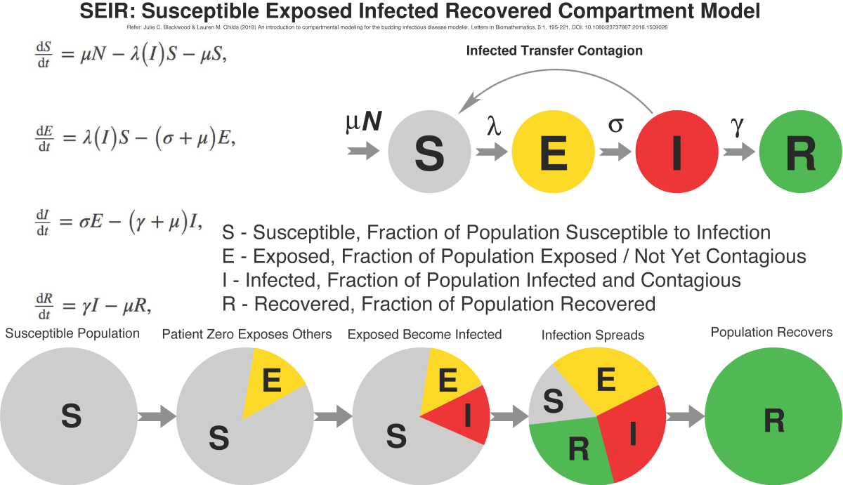
In the SEIR model, it’s assumed that some fixed population is divided into four compartments, each representing a fraction of the population:
- The Susceptible [S] fraction is people yet to be exposed and infected
- The Exposed [E] fraction is people who have acquired the infection but are not yet contagious
- The Infected [I] fraction people who are contagious
- The Recovered fraction those who survived the infection and are immune. Often the latter is labelled as Recovered/Removed [R] if mortality is significant.
A system of four differential equations is used to relate the parameters of the model to the rates (μ, λ, σ, γ) at which the population migrates from one compartment to another. Mathematicians have found analytical solutions, but commonly the problem is solved with software algorithms.
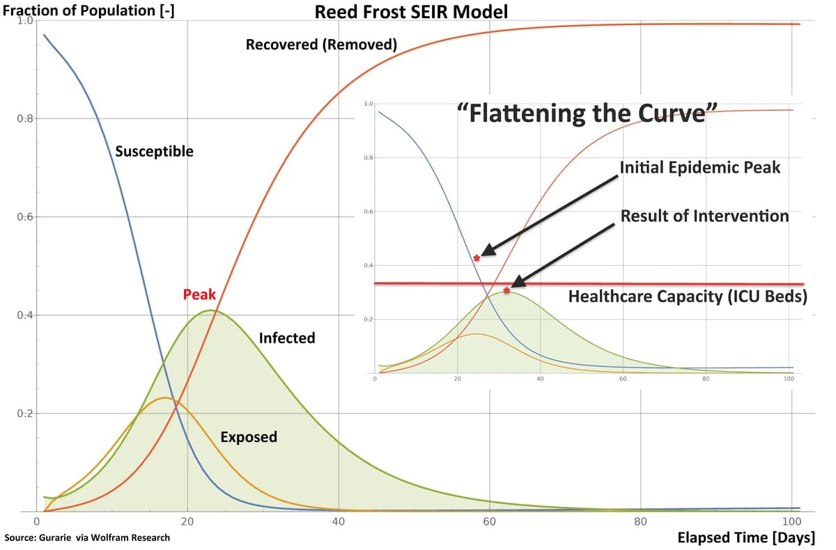
Epidemiologists use models such as SEIR to chart the evolution of an epidemic over time, plotting the sizes of the Exposed, Infected and Recovered fractions of the population. The commonly-seen bell-shaped curve in public presentations is not the symmetrical “normal distribution” curve from statistics; rather, it shows how the Infected fraction of the population steeply grows in size to some peak, and then falls off as the Susceptible population is infected, or protected by some intervention.
An important parameter in epidemic modeling is R0 (“R nought” or “R zero”), or the “basic reproduction ratio”, which is the expected or average number of individuals an infected person subsequently infects. Because R0 is determined by averaging a large number of cases, its size can vary widely, as it depends not only on how contagious the pathogen is, but also on how much contact with others the infected have.
Highly contagious diseases are frequently spread by large or small airborne droplets, and small droplets are usually more contagious, as they persist longer as an aerosol. Many diseases spread via faecal matter, and some pathogens can be aerosolised and spread by flushing toilets.
Another factor is how long a pathogen can survive on surfaces, where a victim might be exposed by touching the surface. A recent US Centers for Disease Control and Prevention report discussing COVID-19 contamination of cruise ship cabins reported traces of the virus detected 17 days after passengers were removed.
The other important consideration is that R0 varies widely with how much contact people have. The more people a contagious individual spends time with, and the longer that time is, the more opportunities the pathogen has to “jump” to a new victim.
The old computer science adage of “garbage in, garbage out” applies. If the data’s wrong, the results will be wrong.
Much has been said in the media about “COVID-19 super-spreaders” who have infected up to dozens – for instance, during community gatherings or choir practice. The important point is that the gathering created the opportunity for increased pathogen spreading, and the individuals labeled as “super-spreaders” might not have been shedding any more of the virus than any other victim of the infection.
The notion of “flattening” the curve by social distancing is no more than reducing opportunities for a pathogen to spread. In effect, the value of R0 is reduced, and the area under the Infected curve in the model is spread over time.
Determining the value of R0 requires much effort, as data must be collected and analysed, and a number of methods can be used. In the early phase of any epidemic this can be challenging, as data may be scarce, incomplete, and replete with errors. This is one reason why many of the early estimates of R0 for COVID-19 varied so widely. As more data is acquired, estimates can become more accurate.
A model is a model
Epidemiological models are no different to any other models, and no matter how precisely the model can describe a situation, the accuracy of the predictions it makes depends critically on the quality of the data put into the model. The old computer science adage of “garbage in, garbage out” applies. If the data’s wrong, the results will be wrong.
This is best illustrated by the ongoing public debate regarding COVID-19 mortality. The virus, like a number of pathogens, can spread via asymptomatic or mildly symptomatic infected individuals, who typically have no idea they’re infected. This is called “cryptic transmission”, and the reason why COVID-19 was able to quietly spread across the globe. The most recent data from Italy and China suggests actual numbers approach 80 per cent.
Accurately estimating the case fatality rate requires that data includes all cases of the disease, as well as the number of dead. During the COVID-19 pandemic, counts of deceased have often been highly inaccurate for many reasons, and counts of total numbers infected have also been inaccurate, with nations counting COVID-19 cases differently.
Where little testing has been done, there may be many cases uncounted or miscounted as asymptomatic, where symptoms had not yet appeared. The resulting estimates are then both inaccurate, and much higher than reality.
The final message is that epidemiological models and the numbers used to populate them must be treated with respect – if we don’t, we might end up spreading fake news.


